session 03: raster metadata and CRS

Affine transforms, pyproj, and aligning our two rasters

Introduction

In Session 01 we opened dem.tif and sentinel.tif for the first time, and mentioned that every raster carries geographic metadata beyond its pixel values: a coordinate reference system and an affine transform. We deferred that metadata so we could focus on simply getting a raster on screen. This session is where we stop deferring it. We look closely at .meta, the affine transform, and the CRS itself, this time reaching for pyproj directly rather than only through rasterio’s convenience wrappers. By the end of this session we will know, precisely, whether our DEM, our Sentinel image, and our vector boundary actually agree on where they are in the world, and we will have a raster_utils.py module that can answer that question for any two files we hand it.

This matters for the solar suitability project specifically because every later factor, slope and aspect from the DEM, land cover from Sentinel, access from the road and power layers, eventually has to be combined pixel by pixel into one suitability map. That is only possible if every layer agrees on where each pixel actually sits on the ground. Getting comfortable with metadata now is what makes Session 07, where we actually force every layer into agreement, make sense later.

Full Raster Metadata

rasterio exposes a dataset’s core metadata as individual attributes, src.width, src.count, and so on, as we already used in Session 01. It also exposes the same information bundled together as a single dictionary, src.meta, which is the form we will reuse most going forward, since it can be passed directly to rasterio.open() when writing a new file, as we will do later in this session.

import rasterio

dem_path = "data/dem.tif"

with rasterio.open(dem_path) as src:
    meta = src.meta
    print(meta)

{'driver': 'GTiff', 'dtype': 'float32', 'nodata': None, 'width': 610, 'height': 605, 'count': 1, 'crs': CRS.from_wkt('GEOGCS["WGS 84",DATUM["WGS_1984",SPHEROID["WGS 84",6378137,298.257223563,AUTHORITY["EPSG","7030"]],AUTHORITY["EPSG","6326"]],PRIMEM["Greenwich",0,AUTHORITY["EPSG","8901"]],UNIT["degree",0.0174532925199433,AUTHORITY["EPSG","9122"]],AXIS["Latitude",NORTH],AXIS["Longitude",EAST],AUTHORITY["EPSG","4326"]]'), 'transform': Affine(0.00026949458523585647, 0.0, -2.5874175128494583,
       0.0, -0.00026949458523585647, 37.14928958559234)}

Each key in this dictionary matters for a different reason. driver identifies the file format, almost always "GTiff" in this course. dtype is the numeric type each pixel is stored as, such as float32 for a DEM with fractional elevation values, or uint16 for raw Sentinel digital numbers. nodata is the value used to mark pixels with no valid data, for example areas outside a sensor’s swath; if this is set incorrectly, or ignored, those pixels will silently pollute any statistic computed later, such as a mean slope. width, height, and count describe the grid shape and number of bands. crs and transform describe where the grid sits on Earth, which is the focus of the rest of this session.

with rasterio.open(dem_path) as src:
    print("Data type:", src.dtypes)
    print("Nodata value:", src.nodata)
    print("Bounds:", src.bounds)

Data type: ('float32',)
Nodata value: None
Bounds: BoundingBox(left=-2.5874175128494583, bottom=36.98624536152465, right=-2.4230258158555857, top=37.14928958559234)

Note

src.bounds returns the geographic extent of the raster as (left, bottom, right, top), in the units of the raster’s own CRS. This is different from src.width and src.height, which are pixel counts, not ground distances. A raster can have the same bounds as another raster while having a completely different width and height, if the two use a different resolution.

Comparing Bounds Between Our Two Rasters

Since the solar suitability project eventually combines the DEM and the Sentinel image, it is worth checking early whether their extents actually overlap in the first place, before worrying about anything more subtle. We can compare bounds directly, as long as both rasters share the same CRS; if they do not, this comparison is meaningless, which is exactly why the CRS check later in this session has to come first in practice.

sentinel_path = "data/sentinel.tif"

with rasterio.open(dem_path) as dem_src, rasterio.open(sentinel_path) as sen_src:
    print("DEM bounds:", dem_src.bounds)
    print("Sentinel bounds:", sen_src.bounds)
    print("DEM CRS:", dem_src.crs)
    print("Sentinel CRS:", sen_src.crs)

DEM bounds: BoundingBox(left=-2.5874175128494583, bottom=36.98624536152465, right=-2.4230258158555857, top=37.14928958559234)
Sentinel bounds: BoundingBox(left=-2.587417512849458, bottom=36.986245361524645, right=-2.423115647383997, top=37.14919975406393)
DEM CRS: EPSG:4326
Sentinel CRS: EPSG:4326

Important

Opening two files at once inside a single with statement, separated by a comma, is a common and convenient pattern. Both dem_src and sen_src close automatically together once the block ends.

The Affine Transform

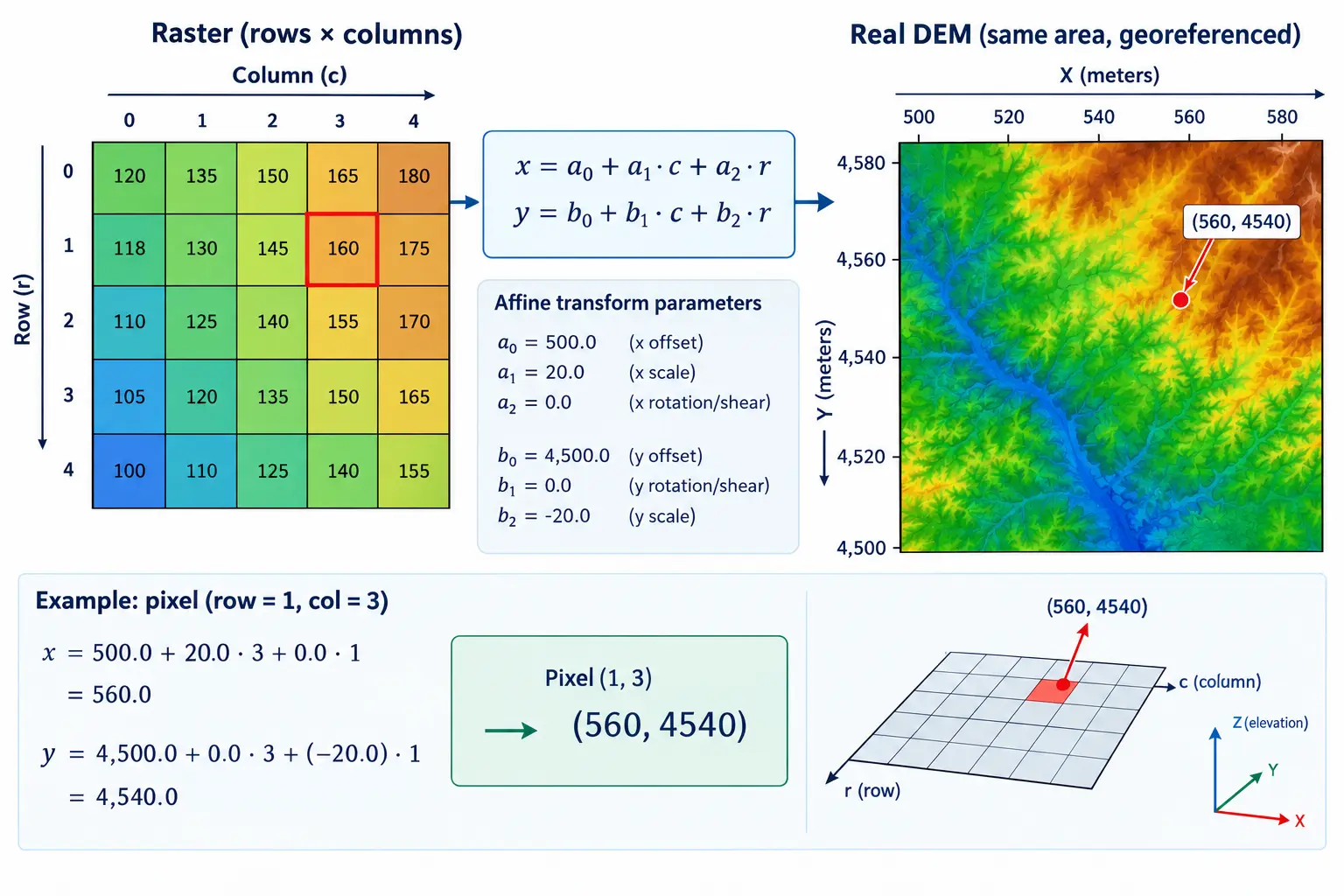
The affine transform is the piece of metadata that turns a pixel’s row and column index into a real-world coordinate, and back. It is stored as six numbers, and rasterio represents it as an Affine object.

with rasterio.open(dem_path) as src:
    transform = src.transform
    print(transform)

| 0.00, 0.00,-2.59|
| 0.00,-0.00, 37.15|
| 0.00, 0.00, 1.00|

Image generated with GPT Image 2.5.

Printed out, an Affine object shows six values, conventionally labeled a through f. a is the pixel width, how many CRS units wide each pixel is in the x direction. e is the pixel height, almost always negative, since raster rows increase downward while y coordinates increase upward. c and f are the x and y coordinates of the top-left corner of the raster. b and d handle rotation, and are 0 for almost every raster we will encounter in this course, including all of ours, since our data is not rotated relative to north.

with rasterio.open(dem_path) as src:
    transform = src.transform
    print("Pixel width:", transform.a)
    print("Pixel height:", transform.e)
    print("Top-left x:", transform.c)
    print("Top-left y:", transform.f)

Pixel width: 0.00026949458523585647
Pixel height: -0.00026949458523585647
Top-left x: -2.5874175128494583
Top-left y: 37.14928958559234

TipNote: resolution from the transform

transform.a and abs(transform.e) give the raster’s spatial resolution directly, the same concept introduced in Session 01. This is a more reliable way to check resolution than assuming it from the file name or documentation, since it comes straight from the file itself.

Converting Between Pixels and Coordinates

rasterio provides two small functions that do this conversion for us, so we rarely need to do the underlying algebra by hand: src.xy() converts a row and column into a real-world coordinate, and src.index() does the reverse, converting a coordinate into the row and column of the pixel that contains it.

with rasterio.open(dem_path) as src:
    x, y = src.xy(0, 0)
    print("Coordinate of pixel (row 0, col 0):", x, y)

    row, col = src.index(x, y)
    print("Pixel containing that coordinate:", row, col)

Coordinate of pixel (row 0, col 0): -2.5872827655568402 37.14915483829972
Pixel containing that coordinate: 0 0

Important

src.xy() returns the coordinate of the center of a pixel, not its corner, by default. This distinction matters when precisely comparing a pixel location against a vector feature, such as checking whether a specific point falls inside a specific DEM cell.

Exercise 1: Locate the center pixel

Open data/dem.tif, find the row and column at the exact center of the raster using src.width and src.height, and print the real-world coordinate of that center pixel using .xy().

Solution

with rasterio.open(dem_path) as src:
    center_row = src.height // 2
    center_col = src.width // 2
    center_x, center_y = src.xy(center_row, center_col)

print(f"Center pixel (row {center_row}, col {center_col}) is at: {center_x}, {center_y}")

Center pixel (row 302, col 305) is at: -2.505086917059904, 37.0677674735585

CRS with pyproj

src.crs, which we already used in Sessions 01 and 02, is actually a rasterio wrapper class, CRS, rather than a raw pyproj object. It behaves similarly for most purposes, but pyproj is the library actually doing the coordinate system work underneath, in rasterio, geopandas, and most of the Python geospatial stack. From this session on, we work with pyproj.CRS directly, since it gives us more detail and is the same object we will need in Session 07 to reproject rasters.

from pyproj import CRS

with rasterio.open(dem_path) as src:
    dem_crs = CRS(src.crs)

print(dem_crs)
print("EPSG code:", dem_crs.to_epsg())
print("Is geographic:", dem_crs.is_geographic)
print("Is projected:", dem_crs.is_projected)

GEOGCS["WGS 84",DATUM["WGS_1984",SPHEROID["WGS 84",6378137,298.257223563,AUTHORITY["EPSG","7030"]],AUTHORITY["EPSG","6326"]],PRIMEM["Greenwich",0,AUTHORITY["EPSG","8901"]],UNIT["degree",0.0174532925199433,AUTHORITY["EPSG","9122"]],AXIS["Latitude",NORTH],AXIS["Longitude",EAST],AUTHORITY["EPSG","4326"]]
EPSG code: 4326
Is geographic: True
Is projected: False

A geographic CRS, such as EPSG:4326, expresses coordinates as longitude and latitude, in degrees, measured on a curved model of the Earth. A projected CRS, such as a UTM zone, flattens that curved surface onto a plane, expressing coordinates in a linear unit, almost always meters. This distinction is the deeper reason .length and .area returned meaningless-looking numbers back in Session 02, when we computed them on geometries built directly in longitude and latitude: those values were in degrees, not meters. Distances and areas are only physically meaningful in a projected CRS.

CRS.from_epsg(4326)

<Geographic 2D CRS: EPSG:4326>
Name: WGS 84
Axis Info [ellipsoidal]:
- Lat[north]: Geodetic latitude (degree)
- Lon[east]: Geodetic longitude (degree)
Area of Use:
- name: World.
- bounds: (-180.0, -90.0, 180.0, 90.0)
Datum: World Geodetic System 1984 ensemble
- Ellipsoid: WGS 84
- Prime Meridian: Greenwich

Tip

CRS.from_epsg() builds a CRS object directly from a known EPSG code, without needing an open file. This is useful any time we need to construct a target CRS by hand, such as when reprojecting a vector layer, as we already did in Sessions 01 and 02 with .to_crs().

Checking Every File Against Every Other File

We now have three files that all need to agree eventually: dem.tif, sentinel.tif, and Desierto_de_Tabernas.gpkg. We already saw, in Session 02, that road.gpkg and power.gpkg did not initially match boundary.crs. It is worth checking our full set of files properly here, rather than assuming.

import geopandas as gpd

with rasterio.open(dem_path) as src:
    dem_crs = CRS(src.crs)

with rasterio.open(sentinel_path) as src:
    sentinel_crs = CRS(src.crs)

boundary = gpd.read_file("data/Desierto_de_Tabernas.gpkg")
boundary_crs = CRS(boundary.crs)

print("DEM:", dem_crs.to_epsg())
print("Sentinel:", sentinel_crs.to_epsg())
print("Boundary:", boundary_crs.to_epsg())

print("DEM matches Sentinel:", dem_crs == sentinel_crs)
print("DEM matches boundary:", dem_crs == boundary_crs)

DEM: 4326
Sentinel: 4326
Boundary: 3857
DEM matches Sentinel: True
DEM matches boundary: False

WarningNote: comparing CRS objects directly

Two CRS objects can be compared with == directly, as shown above, and this is generally more reliable than comparing EPSG codes, since not every CRS has a clean EPSG code. Comparing the raw .to_epsg() values is fine here since both of ours have one, but get in the habit of comparing the CRS objects themselves.

Transforming a Single Point with pyproj.Transformer

Sometimes we need to convert a single coordinate from one CRS to another, without reprojecting an entire file. Transformer.from_crs() builds a reusable converter between two coordinate systems, and its .transform() method converts one coordinate at a time.

from pyproj import Transformer

transformer = Transformer.from_crs(dem_crs, "EPSG:4326", always_xy=True)

with rasterio.open(dem_path) as src:
    x, y = src.xy(0, 0)

lon, lat = transformer.transform(x, y)
print(f"Pixel (0, 0) is at {x}, {y} in the DEM's CRS")
print(f"That is longitude {lon}, latitude {lat}")

Pixel (0, 0) is at -2.5872827655568402, 37.14915483829972 in the DEM's CRS
That is longitude -2.5872827655568402, latitude 37.14915483829972

ImportantNote: always_xy=True

Some CRS definitions traditionally order coordinates as latitude, longitude rather than longitude, latitude. Passing always_xy=True forces pyproj to consistently expect and return coordinates in x, y order, which for a geographic CRS means longitude, latitude. Leaving this out is a common source of coordinates that look plausible but are silently swapped.

This is only a preview. Converting a single point this way is useful for quick checks, such as confirming a pixel’s location on a normal longitude and latitude map, but it is not how we reproject an entire raster. Reprojecting the full DEM or Sentinel image, resampling every pixel onto a new grid, is a more involved operation that we deliberately save for Session 07, once every layer in the project is ready to be aligned at once.

Exercise 2: Where is the DEM’s center pixel, really?

Using the center pixel coordinate you found in Exercise 1, build a Transformer from the DEM’s CRS to EPSG:4326, and print the resulting longitude and latitude.

Solution

with rasterio.open(dem_path) as src:
    dem_crs = CRS(src.crs)
    center_row = src.height // 2
    center_col = src.width // 2
    center_x, center_y = src.xy(center_row, center_col)

transformer = Transformer.from_crs(dem_crs, "EPSG:4326", always_xy=True)
center_lon, center_lat = transformer.transform(center_x, center_y)

print(f"DEM center pixel: longitude {center_lon}, latitude {center_lat}")

DEM center pixel: longitude -2.505086917059904, latitude 37.0677674735585

Quick quiz

Question 1

Why do .length and .area return meaningless values for a geometry built directly in longitude and latitude coordinates?

A. shapely does not support geographic coordinates at all

B. The values are returned in degrees, not meters, since a geographic CRS is not a linear unit

C. shapely always assumes UTM internally

D. The geometry must be invalid

Answer

B. A geographic CRS such as EPSG:4326 measures coordinates in degrees. shapely and geopandas compute .length and .area purely from the numbers they are given, with no awareness of the CRS, so the result is technically correct but expressed in degrees, a unit with no consistent physical length. A projected CRS, in meters, is required for a physically meaningful distance or area.

Multi-band Inspection

sentinel.tif holds several bands stacked together, as introduced in Session 01. Before we calculate anything from them, such as NDVI in Session 04, it helps to inspect each band individually: its description, if the file provides one, and basic statistics.

with rasterio.open(sentinel_path) as src:
    for band_index in range(1, src.count + 1):
        description = src.descriptions[band_index - 1]
        print(f"Band {band_index}: {description}")

Band 1: None
Band 2: None
Band 3: None
Band 4: None

Note

Not every GeoTIFF stores band descriptions; when a file does not, src.descriptions returns None for each band, and the only way to identify a band is by its position, or by comparing basic statistics against known expectations, as we do next.

import numpy as np

with rasterio.open(sentinel_path) as src:
    for band_index in range(1, src.count + 1):
        band = src.read(band_index)
        print(f"Band {band_index}: min={band.min()}, max={band.max()}, mean={band.mean():.2f}")

Band 1: min=0.0, max=5860.0, mean=984.57
Band 2: min=0.0, max=6160.0, mean=1287.08
Band 3: min=0.0, max=6082.0, mean=1539.70
Band 4: min=0.0, max=5826.0, mean=1971.04

This is the same technique introduced briefly in Session 01, now applied deliberately to every band at once. A near-infrared band, for example, typically has noticeably higher reflectance over vegetation than a red or blue band, which is a useful sanity check for confirming band order before relying on it in Session 04.

Plotting DEM and Sentinel Side by Side

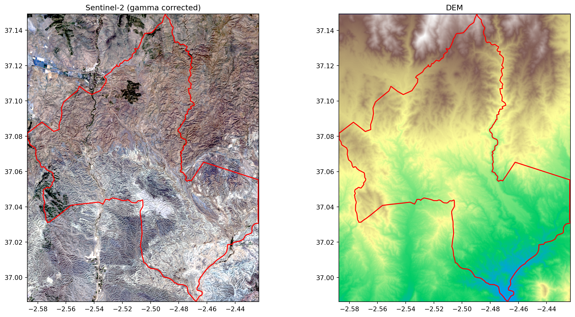
Session 01 plotted the Sentinel image and the DEM separately, each with the study boundary drawn on top. Now that we understand bounds and CRS properly, it is worth placing both rasters side by side in a single figure, which makes any mismatch between them, in extent or in CRS, immediately visible.

rasterio.plot.show, passed a multi-band dataset directly, builds its composite from the raw values of the first three bands with no adjustment. Sentinel-2 reflectance values are naturally low and concentrated in a narrow range, which is exactly why the raw composite in Session 01 looked almost black. A gamma correction stretches that narrow range of dark values back out into something the eye can actually distinguish, without changing the underlying data on disk, only how it is displayed here.

import matplotlib.pyplot as plt
from rasterio.plot import show

boundary = gpd.read_file("data/Desierto_de_Tabernas.gpkg")


def gamma_stretch(band, gamma=0.5):
    """Normalize a band to 0-1 using percentile clipping, then apply gamma correction for display."""
    band = band.astype("float32")
    low, high = np.percentile(band, (2, 98))
    stretched = np.clip((band - low) / (high - low), 0, 1)
    return stretched ** gamma


fig, axes = plt.subplots(1, 2, figsize=(14, 7))

with rasterio.open(sentinel_path) as src:
    boundary_sen = boundary.to_crs(src.crs) if boundary.crs != src.crs else boundary
    rgb = np.dstack([gamma_stretch(src.read(band)) for band in (1, 2, 3)])
    axes[0].imshow(rgb, extent=rasterio.plot.plotting_extent(src))
    boundary_sen.boundary.plot(ax=axes[0], edgecolor="red", linewidth=1.5)
    axes[0].set_title("Sentinel-2 (gamma corrected)")

with rasterio.open(dem_path) as src:
    boundary_dem = boundary.to_crs(src.crs) if boundary.crs != src.crs else boundary
    dem_plot = show(src, ax=axes[1], cmap="terrain")
    boundary_dem.boundary.plot(ax=axes[1], edgecolor="red", linewidth=1.5)
    axes[1].set_title("DEM")

plt.tight_layout()
plt.show()

TipNote: gamma_stretch is a display helper, not a saved product

gamma_stretch only reshapes values for this plot; it is never written back to a GeoTIFF, and nothing about sentinel.tif itself changes. rasterio.plot.plotting_extent(src) gives imshow the same geographic extent show() would have used automatically, which is why the boundary still lines up correctly on top of it.

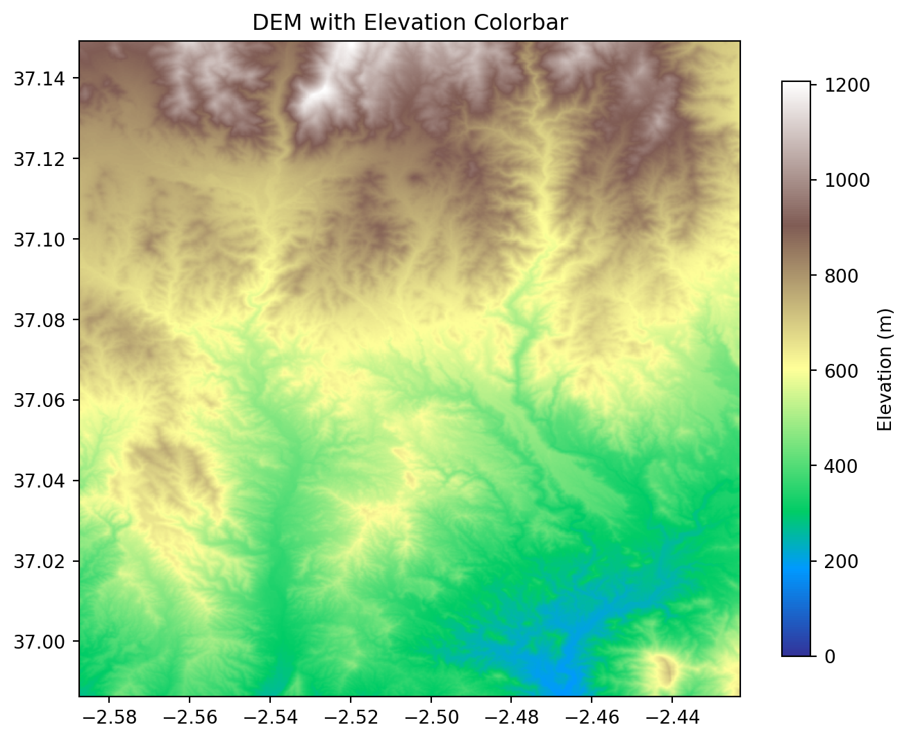
A colorbar is often expected alongside a DEM plot, since, unlike a natural color Sentinel composite, the colors carry no intuitive meaning on their own; a reader needs the scale to know what elevation a given shade of green or brown represents. rasterio.plot.show returns the underlying matplotlib image object, which we can pass directly to plt.colorbar().

fig, ax = plt.subplots(figsize=(8, 8))

with rasterio.open(dem_path) as src:
    dem_image = show(src, ax=ax, cmap="terrain")

im = dem_image.get_images()[0]
plt.colorbar(im, ax=ax, label="Elevation (m)", shrink=0.7)
ax.set_title("DEM with Elevation Colorbar")
plt.show()

Exercise 3: Add a colorbar to a single band

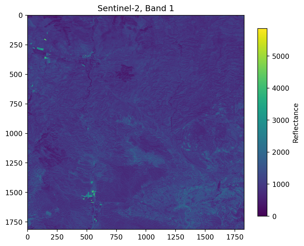
Read only the first band of sentinel.tif as a single 2D array with src.read(1), display it with plt.imshow() using the colormap "viridis", and attach a colorbar labeled "Reflectance".

Solution

with rasterio.open(sentinel_path) as src:
    band_1 = src.read(1)

fig, ax = plt.subplots(figsize=(7, 7))
im = ax.imshow(band_1, cmap="viridis")
plt.colorbar(im, ax=ax, label="Reflectance", shrink=0.7)
ax.set_title("Sentinel-2, Band 1")
plt.show()

Writing a Raster

Every session from Session 04 onward produces a new raster: ndvi.tif, slope.tif, aspect.tif, and eventually suitability.tif. This is the right moment to learn the write side of rasterio, on a small, low-stakes example, before we depend on it for a real output.

The general pattern is to start from an existing file’s .meta, update only the keys that change, such as dtype or count if needed, and pass the result to rasterio.open() in write mode.

with rasterio.open(dem_path) as src:
    dem_array = src.read(1)
    profile = src.profile

cropped = dem_array[:100, :100]

crop_window = rasterio.windows.Window(0, 0, cropped.shape[1], cropped.shape[0])

profile.update({
    "height": cropped.shape[0],
    "width": cropped.shape[1],
    "transform": rasterio.windows.transform(crop_window, profile["transform"]),
})

from pathlib import Path
Path("data/outputs").mkdir(parents=True, exist_ok=True)

with rasterio.open("data/outputs/dem_crop_test.tif", "w", **profile) as dst:
    dst.write(cropped, 1)

print("Saved cropped test raster to data/outputs/dem_crop_test.tif")

Saved cropped test raster to data/outputs/dem_crop_test.tif

ImportantNote: profile versus meta

src.profile is almost identical to src.meta, with a couple of extra keys geared toward writing, such as compression settings. Either works as a starting point; this course uses profile specifically when writing a file, and meta when only inspecting one, purely as a readability convention.

Warning

Cropping an array with slicing, as done above, changes its shape, which means the transform must be updated to match, or every pixel in the new file will report the wrong coordinates. rasterio.windows.transform() computes the correct new transform for a given pixel window. We use this pattern properly, cropping to the full study boundary rather than an arbitrary corner, once we reach clipping in a later session.

Exercise 4: Verify the written file

Open data/outputs/dem_crop_test.tif, the file just written, and print its width, height, and CRS, to confirm it was saved correctly.

Solution

with rasterio.open("data/outputs/dem_crop_test.tif") as src:
    print("Width:", src.width)
    print("Height:", src.height)
    print("CRS:", src.crs)

Width: 100
Height: 100
CRS: EPSG:4326

Building raster_utils.py

This session’s module wraps the metadata and CRS checks above into reusable functions, saved into modules/raster_utils.py. Later sessions, starting with indices.py in Session 04, will import from both data_loader.py and raster_utils.py rather than repeating these steps.

# modules/raster_utils.py

import rasterio
from pyproj import CRS


def get_raster_info(path):
    """Return a dictionary of key metadata for a raster file."""
    with rasterio.open(path) as src:
        info = {
            "width": src.width,
            "height": src.height,
            "count": src.count,
            "dtype": src.dtypes[0],
            "nodata": src.nodata,
            "crs": CRS(src.crs),
            "bounds": src.bounds,
            "transform": src.transform,
        }
    print(f"{path}: {info['width']}x{info['height']}, {info['count']} band(s), CRS {info['crs'].to_epsg()}")
    return info


def check_crs_match(path1, path2):
    """Compare the CRS of two raster files and report whether they match."""
    with rasterio.open(path1) as src1:
        crs1 = CRS(src1.crs)
    with rasterio.open(path2) as src2:
        crs2 = CRS(src2.crs)

    match = crs1 == crs2
    status = "match" if match else "DO NOT match"
    print(f"{path1} and {path2} {status} ({crs1.to_epsg()} vs {crs2.to_epsg()})")
    return match


def save_raster(array, profile, path):
    """Write a NumPy array to disk as a raster, using a given rasterio profile."""
    updated_profile = profile.copy()
    updated_profile.update({
        "height": array.shape[0],
        "width": array.shape[1],
    })

    with rasterio.open(path, "w", **updated_profile) as dst:
        dst.write(array, 1)

    print(f"Saved raster to {path}")

Tip

save_raster assumes a single-band array, which matches every output the rest of this course produces: ndvi.tif, slope.tif, aspect.tif, and suitability.tif are all single-band rasters. It intentionally does not update transform, since it assumes the array has the same extent as the original file the profile was taken from; a cropped array, as in the example earlier in this session, needs its transform corrected separately first.

Summary

This session went beneath the surface of the raster metadata we glossed over in Session 01: the full .meta dictionary, the affine transform and what its six values mean, converting between pixel indices and real-world coordinates, and pyproj.CRS as the library actually responsible for coordinate systems underneath rasterio and geopandas. We confirmed how our DEM, Sentinel image, and study boundary relate to one another in CRS terms, previewed converting a single coordinate between CRS with pyproj.Transformer, inspected each Sentinel band individually, improved our raster plots with colorbars and side-by-side comparisons, and wrote our first raster to disk. We also built modules/raster_utils.py, which the rest of the course will rely on. Session 04 puts all of this to use, calculating NDVI from the Sentinel bands we inspected here and saving it as ndvi.tif with the exact write pattern practiced in this session.